LL(*) grammar analysis

Introduction

The goal of static LL grammar analysis is to compute lookahead expressions that predict alternative productions at any grammar decision point. LL(*) distinguishes between alternative productions using a potentially cyclic DFA where each stop state uniquely predicts an alternative. For example, the following rule is LL(*) but not LL(k) for any fixed k:

x : A* B X
  | A* C Y
  ;

The prediction DFA for rule x is A*(B|C) in regular expression form. Notice that the DFA only predicts which alternative will win. It does not approximate the entire grammar with a DFA. Here, it does not include states to deal with X and Y. The parser will match them after the DFA predicts the appropriate alternative.

The LL(*) algorithm yields an exact DFA when the "lookahead language" is regular (the lookahead language is regular unless the algorithms encounters recursion in the grammar). By exact, I mean that the language generated by the DFA consists of valid and only valid prefixes of phrases in the language generated by the associated grammar.

When the DFA construction algorithm encounters recursive rule invocations in the grammar, it approximates the recursion with cycles in the DFA. For example, the decision for rule s in the following grammar is LL(*) even though the lookahead language is non-regular due to the reference to recursive rule e:

s : e X
  | e Y
  ;

e : L e R
  | I
  ; 

The LL(*) algorithm approximates the nested parentheses (L and R) with cycles. Here is the (minimized) DFA predicting the two productions in rule s. The "s3=>1" notation means state s3 predicts alternative 1.

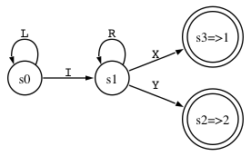
This DFA is a covering approximation in the sense that the DFA generates all valid sequences and some spurious invalid sequence such as IRX. This is no problem (it's still LL(*)) as long as there are no valid or spurious sequences in common between alternatives (the lookahead languages of the alternatives are disjoint within any decision). The spurious sequences only affect when we detect errors. For valid input, the spurious lookahead sequences have no effect upon prediction. It's possible, however, for spurious lookahead sequences to collide. This renders the decision non-LL(*) decision. We resolve this nondeterminism by giving priority to the alternative mentioned first.

To go from grammar to prediction DFAs, we first convert the grammar to a big interconnected NFA and then run a modified "subset construction" NFA-to-DFA algorithm on the NFA.

NFA construction

Because we're converting context free grammars not regular expressions, we need to deal with rule references when building NFAs. For each rule reference, we add two states (p, q) and two epsilon transitions. The first transition goes from state p to the NFA start state for the invoked rule. The second transition goes from the invoked rule's stop state to q. For example, here is grammar with two rule references:

s : a ;
a : A a A
  | B
  ;

And here is the associated NFA (unlabeled edges are epsilon transitions):

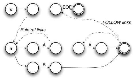
During closure operations, the DFA construction algorithm will traverse the rule invocation transitions and possibly one or more of the "FOLLOW" links emanating from the stop state.

DFA construction

There are two key differences from the usual NFA-to-DFA "subset construction" algorithm.

• we don't pursue any more DFA states if the DFA state we are working on uniquely predicts a single alternative or it detects an ambiguity. The usual algorithm stops when it runs out of NFA states because it wants to represent the entire NFA. We only want to distinguish between alternative productions and let the parser do the actual recognition work.
• even though DFAs don't have stacks, we need a stack to construct an accurate prediction DFA. In a nutshell, the closure operation pushes NFA states as it chases rule invocation links and pops as it traverses rule FOLLOW links to simulate the recursive descent function call.

NFA configurations

The subset construction algorithm represents states in the new DFA by a set of NFA state numbers. Each NFA state number represents a particular configuration of the NFA. The DFA state therefore represents all of the places in the NFA we could be after matching a particular input sequence. In our case, we need to track more information about the NFA configuration. The first thing we need to track is the alternative that a configuration predicts. In the next section, we'll see that we also have to add a stack component to the NFA configuration, but for now let's deal with just state numbers and alternative numbers.

If we built a DFA using the usual algorithm from the following regular grammar, we'd end up with a single accept/stop state that says, "yep, the input matched". It can't tell us anything about the path it took to get to the accept state.

a : A B
  | C D
  ;

To build prediction DFAs, we need to track the alternative numbers as we perform the conversion. Here is the NFA:

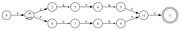
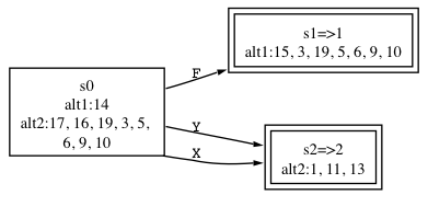
In the DFA, we need to represent an NFA configuration by a tuple: (state, alt), though I've been using notation state|alt (should probably change that to tuple notation but I will stick with the pipes here since many of the DFAs generated by ANTLR will use that notation).

As we begin NFA construction, the start state contains {2|1, 6|2} instead of just states {2, 6}. Since there are no epsilon transitions emanating from either 2 or 6, that is the complete start state. As we continue with construction, the alternative numbers 1, 2 will propagate through to the other DFA states. Here is the DFA we want (loaded with configuration information):

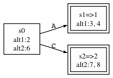
Each DFA state has a name: s0, s1, or s2 and each accept state has =>alt indicating which alternative it predicts. The alt1:... and alt2:... notation lists the NFAs states associated with that alternative (it makes it easier to read than a list of tuples).

The key thing to note is that the algorithm continued beyond the start state because it couldn't uniquely predict alternatives yet--the start state has both alternatives 1 and 2 represented in the same DFA state. In states s1 and s2, on the other hand, it only found NFA configurations associated with one alternative (alternatives 1 and 2, respectively). It makes these accept states and doesn't consider them further. That is how it knows not to continue on to the B and D edges.

We only want to put a DFA state onto the work list for further processing if it has multiple alternative numbers and that state does not represent an ambiguity in the grammar.

Detecting ambiguities

Consider the following ambiguous grammar

a : A
  | A
  ;

and its NFA:

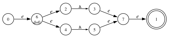
Our start state, s0, has two NFA states (one for each alternative): {2|1, 4|2}. From s0 on A, we can reach NFA states 3 and 5, which gives us a new DFA state with initial contents: {3|1, 5|2}. Adding in the closure, gives us a problem. The DFA state has the following NFA configurations: {3|1, 7|1, 1|1, 5|2, 7|2, 1|2}. Uh oh. We can reach the same NFA states, 7 and 1, from two different alternatives. That means we found two paths through the grammar that reach the exact same spot. The algorithm has detected an ambiguity (note: this is not merely an LL(*) nondeterminism--it's a grammar ambiguity). We can report a static analysis error to the user and resolve the ambiguity by choosing the first alternative. In the following DFA generated by ANTLR, you'll see the NFA configurations associated with alternative 2 have been turned off (we turn on the resolved bit).

In this way, there is a single predicted alternative and we can label s1 an accept state that predicts alternative 1.

Dealing with rule references

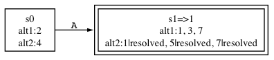
Rule references in a grammar become epsilon transitions pointing to the NFA created for the target rule. The stop state for the target rule has an epsilon transition back to the state following the rule invocation state. Consequently, without using a stack during DFA construction, we would get prediction DFAs that allow invalid lookahead sequences (even in non-recursive grammars). Because these spurious lookahead sequences might collide between alternatives, we'd unnecessarily claim we couldn't distinguish between the alternatives. Consider the following grammar that references a nullable rule b:

a : b X
  | b Y   
  ;

b : F     
  |       
  ;

To compute even LL(1) lookahead for rule a, we need to track context information. In other words, FIRST(b X) is {F,X} not {F,X,Y}. From the first alternative, we can only return to one rule invocation location not both. To compute FIRST, we can use a simple depth first walk of the NFA looking for the first visible token-labeled transitions:

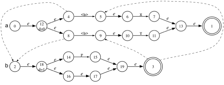
Since rule b is nullable, we reach b's stop state, which has two "FOLLOW" links. Because we started the FIRST computation in a's first alternative, we should only chase the epsilon transition leading to the NFAs state before X. If we followed both transitions, we'd find both X and Y, leading to an incorrect FIRST set. We need a stack to track from which state we enter a rule so that we can return to the right spot in the invoking rule's NFA.

The only wrinkle for LL(*) is that we need a stack associated with every NFA configuration. Since we are collecting and processing these configurations later, each configuration needs its own stack kind of like storing a continuation. (Presumably a functional language could deal with this more naturally). The configuration tuple now looks like state|alt|context. We can omit the context component if it's the empty stack [$]. Here is the DFA predicting the alternatives of rule a:

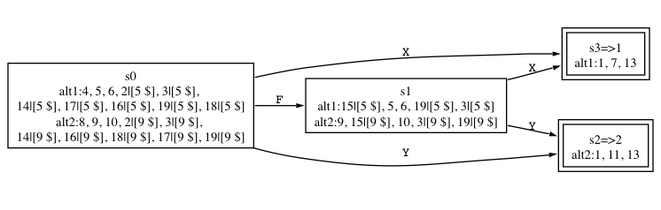
The bracketed sequences shown in the DFA states are stack components of NFA configurations. For example, the start state begins with a kernel of {4|1, 8|2} and then computes closure. The closure operation beginning at 4|1 immediately jumps to the state 2, the start state of rule b. When it adds state 2 for alt 1, it also records the return state: 5. So, the proper NFA configuration for this move is 2|1|[5 $]. (Since the diagram organizes configurations by alternative number, you see only 2|[5 $].) Continuing with the closure operation, we add configurations for NFA states 14, 16, 17, 19, and then finally reach 3, the stop state of b. Rather than following all possible epsilon transitions, we pop 5, the return state, from the context stack and continue among the NFA states for rule a.

The only time we chase all FOLLOW transitions is when we have no context information (nobody called this rule). This is what happens when we compute the prediction DFA for rule b:

The prediction can see both X and Y in rule a (it's FOLLOW(b)) and so that set predicts the second, empty alternative of b.

Recursive rules

I'll leave this discussion out at the moment, though the algorithm handles recursion properly.

Stack representation

Each NFA configuration needs a state stack so closure operations can follow the appropriate link back to an invoking rule's NFA. To make this more efficient, we can share stack elements using a tree. (Similarly, if we track all function calls made by a running program, we end up with a tree.) The complete context for an NFA configuration is the set of states on the path from a node to the root. For example, here's a sample NFA context tree representing stacks for multiple configurations.

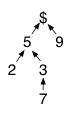
The most obvious stacks are the longest chains (stack top is on the left and $ means EOF):

• 2 5 $
• 7 3 5 $
• 9 $

To get stacks that big, however, we had to have configurations that used the intermediate nodes as stack tops:

• 5 $
• 3 5 $
• $ (empty stack and our initial condition)

The trees only have parent pointers rather than child pointers because we are always walking back up the tree to pop nodes off. We never walk the tree downwards from the $ root.

To "push" an NFA state s onto the context stack with stack-top/leaf-node c, we create a new node holding s and with parent pointer pointing at c: new NFAContext(c, s). To "pop" a state from the stack, we simply set the current context c to point to c.parent.

NFA Configuration stack context comparison

Two NFA configurations indicate a grammatical ambiguity when they refer to the same state but for different alternatives and with the same context; e.g., (s|i|ctx) and (s|j|ctx). That means that we can get to the same place in the grammar following the same path in more than one way. It turns out that the context comparison is tricky. We can't just compare for equality, where one stack is exactly the same as another (the two paths up to the context tree root are the same). We also have to check to see if:

• one of the contexts is empty or
• one stack is a suffix of the other

Empty and non-empty contexts

When comparing contexts, if one is empty and the other has a stack, then they should be considered the same context otherwise we will miss some ambiguities. This can only happen when a closure reaches a rule stop state without a call stack and re-enters the rule from another. Clearly, to be in a rule, someone has to call it so there is a context. We just don't know what it is statically. Consequently, an empty stack actually means "don't know", not empty. One of the rule references has to be the invoking context and, if we reach the stop state, we will positively get back to the same context (we chase all FOLLOW transitions when we have no context information). Reaching the same state with and without context implies that we got back to the same state twice from the same context--a missing context is like a wildcard. I'm pretty sure that's the intuition behind this. Anyway, an example makes it clear that we need it.

In the following grammar, rule s has a + loop that can match an A by following the epsilon loopback transition (alt 2) or by reaching the stop state for s (alt 1).

s : A+ ;
x : s s ;

Since we began the closure operation inside s, no one "called" it and therefore we have no context. The loopback state 7 reaches the start of the loop, state 4, as you can see in the NFA for s (couldn't get DOT to show this properly...sorry):

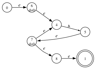
State 7 can also reach 8 and then the stop state, 1. From the stop state, it chases all FOLLOW transitions to states 10 and 12 in the NFA for rule x:

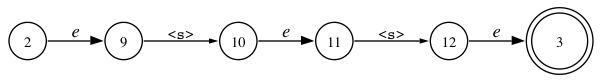
State 10 then goes through 11 back to the start of rule s, state 0. From 0, we go through 6 and then to 4. We have reached state 4 with context [12 $] because the return state is 12.

So, we have two configurations: 4|2|[$] and 4|1|[12 $]. We can reach the same place in the grammar by staying in rule s and also by falling off the end of s and reentering s via rule x. We need to see this situation as an ambiguity because the grammar is ambiguous for input A. We can match A by staying in the loop or by falling off the end of s, going back to x, and then back into s to match A. Here is the DFA with all of the NFA configurations:

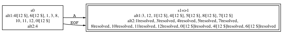
Also, let me also point out that start state, s0, has conflicting configurations also (4|1|[12 $] and 4|2|[$]). We never issue ambiguity warnings for the start state. We let it continue for one more edge so that we can give sample ambiguous input to the programmer in an error message. (Once we have ambiguous configurations, that condition will persist as we expand the DFA along that path.)

Stack suffixes

The other case where two contexts are similar even when not equal, is when one is a suffix of the other. A suffix is a list of elements of any length starting from the top of the stack. In other words, for stack

$,

is a stack suffix.

For example, contexts [21 12 $] and [21 9 $] are not equal and neither is the suffix of the other. But, [21 $] and [21 12 $] are "the same" because 21 is a stack suffix of [21 12 $].

Here's a few more examples:

• [$] suffix any context
• [21 $] suffix [21 8 $]
• [21 8 $] suffix [21 $]
• [21 18 $] suffix [21 18 8 9 $]
• [21 18 8 9 $] suffix [21 18 $]
• [21 8 $] not suffix [21 9 $]

Once

is the top of both stacks, closure operations either leave the stack alone or add elements, yielding larger identical suffixes on top of the stack. If we reach a rule stop state, we might pop one element off of the stack, shrinking suffix

by one. If we pop

all the way off, we reduce the contexts to: $ and

$. So, if one stack is a suffix of another, future closure operations will either leave context alone, increase its size, or degenerate to the empty versus nonempty stack condition in the previous section.

Without this definition of context similarity, the LL(*) algorithm would sometimes not detect ambiguities soon enough (it would process too much of the NFA). Seems to me the if-then-else ambiguity was a good example if the else-clause were in a different rule.

Ok, on to the algorithm itself.

Algorithm

createDFA:
    add start-state to states as unmarked
    while there is an unmarked dfa state d:
        mark d;
        for each input symbol a:
            t = closure(reach(d, a))
            if t is already in states:
                t = existing state
            else:
                if ambiguous-alts(d)>0:
                    set resolved bit in non-min configs
                    set each config alt to min alt number in d
                if configs of t predict single alt, add as marked accept state
                else add t as unmarked state
            transition[d, a] = t

start-state:
    for each edge, e, of s0:
        add config(e.target, alt-num, $) to start-state

reach(d, a):
    d' = new DFA state
    for each config c of d:
        for each transition t of c.state:
            if not c.resolved and transition t.label==a:
                add config(t.target, c.alt, c.context) to d'
    return d'

closure(d):
    for each config c in d, add closure(c.state, c.alt, c.context) to d

closure(d, c):
    if busy list contains c, return
    add c to busy list
    add c to result
    if alt is rule stop state, add ruleStopClosure(d,c) to result
    else add commonClosure(d,c) to result

commonClosure(d, c):
    for each rule transition edge e of s:
        context' = c.context
        if e.target is current rule start state or e.target in context:
            set c.context.recursed
        else context' = context(c.context, e.return-state)
        add closure(d, config(e.target, alt, context')) to result
    for each non rule transition epsilon edge e of s:
        add closure(d, config(e.target, alt, c.context)) to result

ruleStopClosure(d, c):
    if !c.context.recursed:
        if context empty, commonClosure(d, c)
        else add closure(d, config(c.context.returnState, c.alt, c.context.parent)) to result
    else:
        invokingRule = c.context.returnState.rule;
        for all epsilon edges e not leading to NFA state in invokingRule:
            add closure(d, e.target, altNum, context) to result
        for the only edge e pointing at context.returnState:
            add closure(d, config(e.target, c.alt, c.context)) to result

ambiguous-alts:
    return set containing all i and j for all config pairs (s|i|ctx1) and (s|j|ctx2)
        where ctx1==ctx2 or
              ctx1 is stack suffix of ctx2 or
              ctx2 is stack suffix of ctx1 or
              either ctx1 or ctx2 is empty